Magnetic Fields

Field of a Magnetic Dipole

So far we have not talked about sources of magnetic fields, but even in our discussion of magnetic forces, we have not made any mention of magnetic charges that behave in magnetic fields the same way that electric charges behave in electric fields – with forces that act along the field lines, rather than perpendicular to them. We don’t have the equivalent of Coulomb’s law for two magnetic point charges, for example. Let’s explore this possibility here:

From our experience, we know that if we put two magnets together a certain way, they stick together, and if we turn one of them around, they repel. So they clearly have a directionality to them. The closest analogy in electricity is a dipole. Indeed, if we put two dipoles end-to-end one way, they will attract, and if we turn one of them around, they will repel.

The attraction and repulsion occur because the there is a field created by one dipole that points in the direction outward from the positive charge, and the field gets weaker with distance, so the other dipole will feel a net force according to whichever of the two charges is closer to the dipole creating the field. In magnetism, we call the end of the magnet from which emerges the outward-going field lines the north pole, and the end into which the field lines converge the south pole. From the figures above, it’s clear that the dipoles whenever like poles are brought together, and attract when opposite poles are brought together. What’s even weirder is that every time we cut a magnet with two poles into two pieces, we just get two more magnets with two poles.

If we examine the the field lines for a bar magnet closely and compare them to an electric dipole field, we see how fundamentally-different the two fields are. For the electric dipole, the field changes direction between the two poles, while for the magnetic case, the field lines continue straight through:

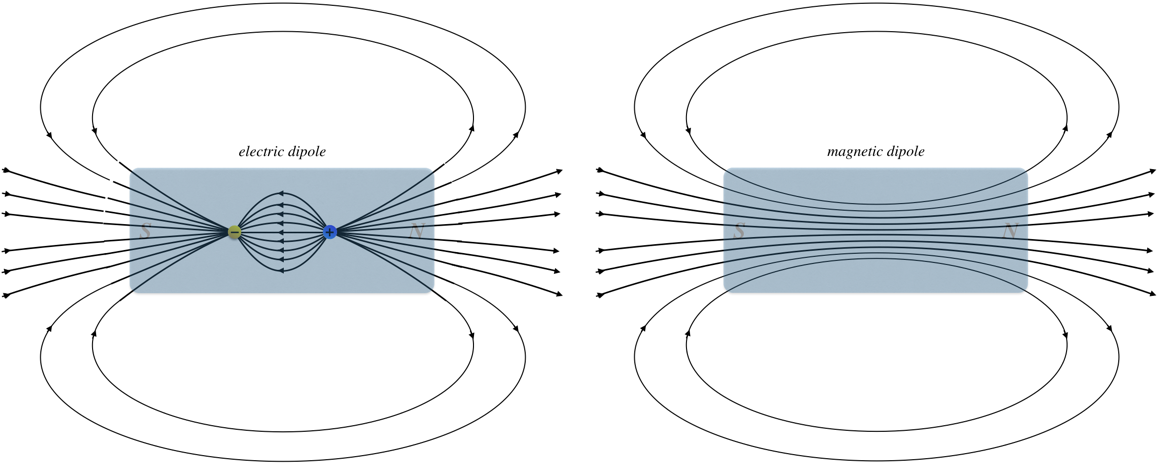
Outside the dipoles, the fields look the same, but they are clearly different, which we can characterize in the following way: Magnetic field lines always form closed loops, while electric field lines begin and end on electric charges.

Put another way, unlike electric fields which form their dipole fields from two monopoles, there don’t seem to be any magnetic monopoles. Or at least we have never been able to detect a magnetic monopole, despite many decades of experimental search for them. It turns out that electromagnetic theory doesn’t exclude the possibility of the existence of these point charges of magnetism, but ultimately our theories have to agree with what we observe in experiments, so at least for the moment (and for the duration of this class), we will maintain the position that they simply don’t exist.

Gauss’s Law for Magnetism

The revelation that our theory of magnetism doesn’t include individual magnetic charges has an immediate consequence for the magnetic equivalent of Gauss’s law. With magnetic field lines always forming closed loops, any field line that penetrates a Gaussian surface going in one direction (say going into the volume bounded by the surface) must later emerge from that closed surface later in order to form the closed loop. If there is a field line exiting a surface for every field line that enters it, then the net flux must necessarily always be zero. Of course, from Gauss’s law, this means that there can never be any charge enclosed, and this makes sense, given that there is no magnetic charge. Mathematically, we express this Gauss’s law for magnetism in either integral or local form: \(\oint \overrightarrow B\cdot d\overrightarrow A = 0\;,\;\;\;\;\; \overrightarrow \nabla \cdot \overrightarrow B = 0\)

Field of a Moving Point Charge

When we first started discussing magnetism, we noted a force between two current-carrying wires. From there, we focused on the fact that a magnetic field affects only moving electric charges, but it should be equally clear that the source of a magnetic field must also be moving electric charges. One might object that we just said that magnetic fields don’t have point sources, so what difference does it make that we insist that the point source be moving? We will see that this makes all the difference, because this leads to a field that doesn’t point directly toward or away from that charge – the direction of the field is determined by the direction of the velocity vector.

As different as the magnetic field is from the electric field, there are still so many striking similarities that it is useful to describe the features of the magnetic field from a moving point charge in parallel with the Coulomb electric field. This magnetic analog of the Coulomb field is called the law of Biot & Savart (Biot-Savart law for short).

---

Feature Coulomb Biot-Savart $|\overrightarrow{E}| \propto q\; \text{(charge)}$ $|\overrightarrow{B}| \propto q |\overrightarrow{v}| \; \text{(moving charge)}$ $|\overrightarrow{E}| \propto \dfrac{1}{r^2}$ $|\overrightarrow{B}| \propto \dfrac{1}{r^2}$ $\overrightarrow{E} \parallel \overrightarrow{r}$ $\overrightarrow{B} \parallel \overrightarrow{v} \times \overrightarrow{r}$ $\overrightarrow{E} = \left( \dfrac{1}{4\pi\epsilon_o} \right) \dfrac{q \overrightarrow{r}}{r^3}$ $\overrightarrow{B} = \left( \dfrac{\mu_o}{4\pi} \right) \dfrac{q \overrightarrow{v} \times \overrightarrow{r}}{r^3}$ ————- ————————————————————————————————— ———————————————————————————————————————–

The physical constant that makes the units work out for the force is called the magnetic constant (permeability of free space) which has values of $\mu_o = 4\pi\times 10^{-7} \frac{T\cdot m}{A}$.

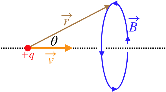
While it is not obvious from the final form of the equation for the magnetic field, the resulting field is a circle centered at the line passing through the charge along the direction of motion.

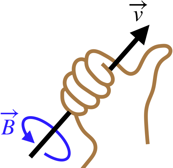
Rather than using the right-hand-rule for the cross-product $\vec v \times \vec r$ (which gives the direction of the magnetic field at a specific point in space), we can get a bigger-picture idea of the magnetic field lines by using a different right-hand-rule: Point the thumb of the right hand in the direction of motion of the charge, and the magnetic field direction everywhere in space forms closed circles around the line of motion in the direction that the fingers curl as shown in the figure below.

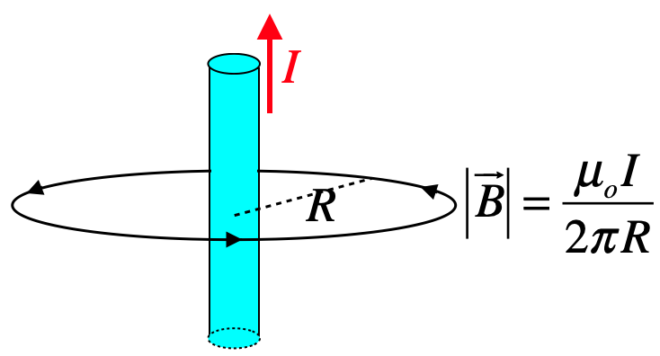
Field of a Current-Carrying Wire

It is far more common to have physical situations where a magnetic field is created by a current-carrying wire than by a point charge. Fortunately, we already know how to convert from moving point charges to current elements: \(I\;\overrightarrow {dl} \leftrightarrow dq \;\overrightarrow v\) We therefore get this for a line of current from the law of Biot-Savart: \(\overrightarrow B = \int d\overrightarrow B = \int\left[\left(\dfrac{\mu_o}{4\pi}\right)\dfrac{I}{r^2}\overrightarrow {dl} \times \widehat r\right] = \dfrac{\mu_o}{4\pi}\int \dfrac{I{\overrightarrow{dl}} \times \overrightarrow r}{r^3}\)

Magnetic Field of a Long Straight Wire

One of the key differences between computing magnetic fields and electric fields is that while we were able to use symmetry to help us solve for components of the electric field, in the case of the magnetic field, this is much harder to do, and is much safer to just get all the vectors right and trust vector math thereafter.

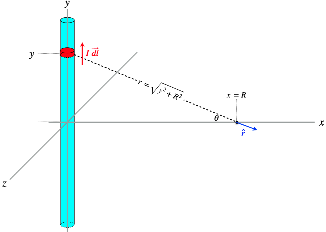
We start by expressing all the relevant quantities in terms of our chosen coordinate system:

---

$\overrightarrow{dl} = dy$ $\widehat{j}$ $\widehat{r} = \cos\theta \; \widehat{i} - \sin\theta \; \widehat{j}$ $\cos\theta = \dfrac{R}{\sqrt{y^2 + R^2}}$ —————————————— ———————————————————————– ——————————————–

Next, write down Biot-Savart’s law for the current element, and simplify: \(\begin{aligned} d\overrightarrow B && = \left(\dfrac{\mu_o}{4\pi}\right)\dfrac{I}{r^2}\overrightarrow {dl} \times \widehat r \\ &&= \left(\dfrac{\mu_oI}{4\pi}\right)\dfrac{dy}{y^2+R^2}\widehat j \times \left(\cos\theta\;\widehat i - \sin\theta\;\widehat j\right) \\ &&= \left(\dfrac{\mu_oI}{4\pi}\right)\dfrac{dy}{y^2+R^2} \left(\cos\theta\;{(-\widehat k)} -0\right) \\ &&= \left(\dfrac{\mu_oI}{4\pi}\right)\dfrac{dy}{y^2+R^2}\left(\dfrac{R}{\sqrt{y^2+R^2}}\right)\left(-\widehat k\right) \\ &&= \left(\dfrac{\mu_oI\;R}{4\pi}\right)\dfrac{dy}{\left(y^2+R^2\right)^{\frac{3}{2}}}\left(-\widehat k\right) \end{aligned}\) All that remains is to add up the contributions to the field from all the current elements, which means integrating this from $y=-\infty$ to $y=\infty$ \(\begin{aligned} \overrightarrow B && = \left(-\widehat k\right)\left(\dfrac{\mu_oI\;R}{4\pi}\right) \int\limits_{-\infty}^{+\infty} \dfrac{dy}{\left(y^2+R^2\right)^{\frac{3}{2}}} \\ && = \left(-\widehat k\right)\left(\dfrac{\mu_oI\;R}{4\pi}\right) \left[\dfrac{1}{R^2}\;\dfrac{y}{\sqrt{y^2+R^2}}\right]_{-\infty}^{+\infty} \\ && = \left(-\widehat k\right)\left(\dfrac{\mu_oI}{4\pi R}\right)\left[2\right] \\ && = \left(\dfrac{\mu_oI}{2\pi R}\right)\left(-\widehat k\right) \end{aligned}\)

As with the electric field, the magnetic field obeys superposition, which means we can combine the result of this physical situation with others to get a net magnetic field. It is also worth noting that both the moving point charge and the long, straight wire yield magnetic fields whose line close back on themselves (form closed loops) – in nether case does a field emanate out of or into the source. There are no magnetic monopole fields.

Field of a Loop

Another useful field to know is that which points along the axis of a circular loop of current. The method is essentially the same as above, but the coordinate system used is different, which leads to a little bit more complicated vector manipulation.

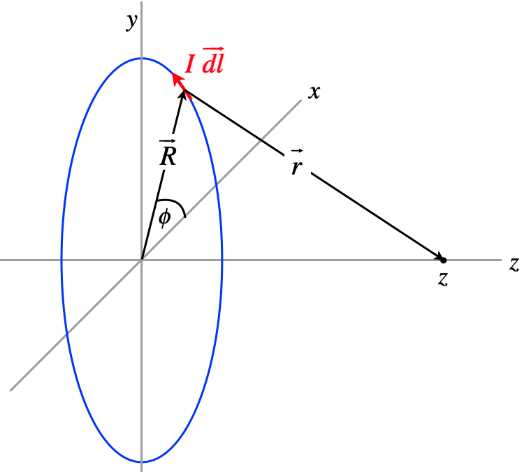
Again start by expressing quantities in terms of the coordinates we have set up. We can again write everything in terms of the basis vectors. First we have the magnitude of the segment of wire: \(\left|\overrightarrow{dl}\right| =R\;d\phi\) Next we note that tail-to-head vector addition gives: \(\overrightarrow R + \overrightarrow r = z \widehat k\;\;\;\Rightarrow\;\;\; \overrightarrow r = - \overrightarrow R + z \widehat k\) Before we can integrate using the Biot-Savart law, we have to resolve the vector products. Looking at the diagram, we can see that the current element $\overrightarrow{dl}$, the position vector of the current element $\vec R$, and the unit vector $\hat k$ are all mutually orthogonal, making $\vec dl \times \vec R$ parallel to $\hat k$, and $\vec dl\times \hat k$ parallel to $\vec{R}$. This allows us to use the right-hand rule to complete these products \(\overrightarrow{dl}\times\overrightarrow r=\overrightarrow{dl}\times\left(-\overrightarrow R + z\widehat k\right) = R\;dl\;\widehat k + z\;dl\;\widehat R\) Putting this result into the integral and noting that magnitudes of the vectors $\vec{r}$ and $z\hat k$ are constant in the integral, and satisfy $r^2=R^2+z^2$, we get: \(\overrightarrow B = \dfrac{\mu_oI}{4\pi} \int \dfrac{\overrightarrow{dl}\times\overrightarrow r}{r^3} = \dfrac{\mu_oI}{4\pi\left(R^2+z^2\right)^{\frac{3}{2}}}\int \left[R\;dl\;\widehat k +z\;dl\;\widehat R\right]\) While the magnitude of $\vec{R}$ doesn’t change over the integral, its direction does change, so we have to write the unit vector $\hat{R}$ in terms of the coordinates to do the integral of the second term. Let’s do each integral separately. The first is straightforward, since the integral of just dl is simply the circumference of the circle: \(\begin{aligned} \dfrac{\mu_oIR}{4\pi\left(R^2+z^2\right)^{\frac{3}{2}}}\widehat k\int dl = \dfrac{\mu_oIR^2}{2\left(R^2+z^2\right)^{\frac{3}{2}}}\widehat k \\ \dfrac{\mu_oIz}{4\pi\left(R^2+z^2\right)^{\frac{3}{2}}}\int dl \widehat R = \dfrac{\mu_oIz}{4\pi\left(R^2+z^2\right)^{\frac{3}{2}}}\int \limits_0^{2\pi} R\;d\phi \left(\cos\phi\;\widehat i + \sin\phi\;\widehat j\right)=0\end{aligned}\) The second integral just ends up vanishing, giving the result for a magnetic field along the axis of a loop of radius $R$ a distance $z$ from the plane of the loop: \(B = \dfrac{\mu_oIR^2}{2\left(R^2+z^2\right)^{\frac{3}{2}}}\) If we are only interested in the field at the center of the loop, we plug in $z=0$ to get the simple result: \(B = \dfrac{\mu_oI}{2R}\)

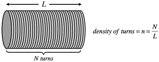
Field of a Solenoid

It is possible to stack lots of individual dipoles on top of each other to create a long tube called a solenoid. Such a device consists of a number of turns in the coil $N$, and a length $L$, resulting in what will be the critical measure, the turn density:

To compute the field,like the loop, we will only look on the axis. But we will also simplify it further by assuming we are looking at a point on the axis inside the solenoid far from the ends (so essentially it has an infinite length, though the turn density is of course finite).

We treat this as a collection of an infinite number of loops. If we pick an origin (which we can place anywhere along the infinite axis), then we have the field at that point by a loop at a position $z$ on the axis is given by equation 19 above. Then we need to add up the field contributions at the origin due to all of the loops. The problem is, there is not a loop at every point along the z-axis. With a turn density of $n$, the number of turns in a tiny slice $dz$ would be $ndz$. The total current in that slice would then be this number multiplied by the current through the wound wire (I): \(\text{current in a } dz \text{ slice located at } z = I\;n\;dz\) Plugging this into Equation 19 for the current, gives the tiny contribution to the field by the slice, and adding them all up gives the field. We are not given the radius of the solenoid, but we will call it $R$ (which turns out to be useless): \(B = \int\limits_{-\infty}^{+\infty} \dfrac{\mu_o\left(n\;I\;dz\right)R^2}{2\left(R^2+z^2\right)^{\frac{3}{2}}} = \dfrac{\mu_o\;n\;I\;R^2}{2}\int\limits_{-\infty}^{+\infty} \dfrac{dz}{\left(R^2+z^2\right)^{\frac{3}{2}}} = \dfrac{\mu_o\;n\;I\;R^2}{2}\left[\dfrac{z}{R^2\sqrt{R^2+z^2}}\right]_{-\infty}^{+\infty}=\mu_o\;n\;I\) 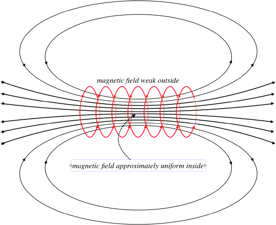There are a few particularly interesting aspects of the fields of solenoids:

1. The field within the solenoid doesn’t change much (it is pretty much uniform). This basically comes from the fact – as we found here – that the field on the axis doesn’t depend upon the radius of the solenoid.

2. The field just outside the solenoid (on its side, not the end) is very weak (basically it is zero).

3. The field looks just like that of a bar magnet, but it can be turned on and off by switching the current on or off.

Ampére’s Law

A Magnetic Analog to Gauss’s Law for Electricity

We have already stated that Gauss’s law for magnetic field is trivial, as there are no magnetic monopoles, but it turns out that there is a separate mathematical law that works for magnetic sources in the same way that Gauss’s law works for electric sources. It incorporates "enclosed" sources, and allows us to use symmetrical situations to solve for fields using methods simpler than integrating Biot-Savart’s law.

This magnetic version of the electrical Gauss’s law is called Ampére’s law, and since it can’t involve enclosed point sources, it instead deals with lines of current, which either circle back on themselves to form a closed circuit, or are infinitely-long (and circle-back on themselves at infinity). But how do we "enclose" a line of current? In the case of charge, it was enclosed if there was no way to remove the charge from the Gaussian surface without breaking through the surface (i.e. the surface has no holes in it). In the case of Ampére’s law, we consider a current to be enclosed by an imaginary closed path – called an Ampérian circuit – rather than a surface. Such a current is enclosed when there is no way to move the line of current out without it breaking through the Ampérian circuit.

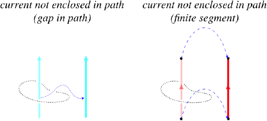
There are two ways that a current won’t be enclosed: If there is a break in the path around the wire, so that the wire can slide through it, or is the segment of wire is finite in length and does not form a closed loop. If the loop of wire is closed, then the Ampérian circuit is "linked" with it, and the current is enclosed. If the wire is infinitely long, the wire similarly cannot escape the Ampérian circuit without breaking through it, so its current is also enclosed. [Mathematically, we generally define a current to be "enclosed" by a closed path if it pierces every possible surface that is bounded by the closed path. Clearly there are stretched surfaces we can construct with the closed path as it border that do not allow a finite-length segment to pierce it.]

\(\oint \limits_{\rm {path}}\overrightarrow B \cdot \overrightarrow {dl} = \mu_oI_{enclosed}\) The integral is performed along any Ampérian circuit that goes completely around the enclosed current, in the same way that the integral for Gauss’s law works for any closed surface that encloses the charge. All of the properties of Gauss’s law have analogous properties for Ampére’s law:

1. Enclosed is defined in terms of ability to remove charge/current from surface/closed path without breaking through the enclosure.

2. The sign of the charge inside a Gaussian surface is related to the positive direction of the area vector. If the total flux is in the negative direction (opposite to the area orientation), then the enclosed charge is negative. Similarly, we define a positive direction of circulation for an Ampérian circuit, and if the direction of the magnetic field of the current has the same circulation orientation as that of the Ampérian circuit, then that current is "positive," otherwise it is "negative."

3. There can be both positive and negative charges/currents enclosed in a surface/closed path, and these are combined to give a net charge/current.

4. We can use symmetry to solve for a field. This usually means that the field is either parallel or perpendicular to the surface/closed path, and that it has a constant magnitude on that surface/closed path.

5. The shape of the surface/closed path is not relevant, as long as it is closed.

Applications of Ampere’s Law

You can read how Ampere’s law is applied in various current distributions at the following link:
https://physics.kebede.org/assets/notes/magnetism/field/ampere/applications.pdf